Heterogeneous Graph and Knowledge Graph

1. Heterogeneous Graphs

Definition

G = (V, E, R, T)

V : set of nodes, which have their types in set T

E : set of edges, which have their relations type in set R

R : set of relations

T : set of nodes’ type

2. Relation GCN

Formulation

$$
h_v^{(l+1)} = \sigma(\sum_{r \in R}\sum_{u\in N_v^r}\frac1{c_{v,r}} W_r^{(l)}h_u^{(l)}+W_0^{(l)}h_v^{(l)})
$$

Scalability

Block Diagonal Matrices

use B low-dim matrices to present $W_r^{(l)}$, which reduce parameters from $d^{(l)}\times d^{(l+1)}$ to $B\times \frac{d^{(l+1)}}B \times \frac{d^{(l)}}B$

Basis Learning

regard $W_r^{(l)} = \sum_{b=1}^B a_{rb}^{(l)}\cdot V_b^{(l)}$ , where $V_b^{(l)}$ is shared and each relation need only learn ${a_{rb}^{l}}$

3. RGCN For Link Prediction

Training

1. Split edges into training message edges, training supervision edges, validation edges and test edges
2. use RGCN to score the training supervision edges
3. create negative edges by perturbing the training supervision edges
4. use RGCN to score the negative edges
5. max the score of training supervision edges while min the score of negative edges

Evaluation

1. calculate the score of test edges
2. calculate the score of negative edges, which produced by perturbing the test edges and not belong to training message edges and training supervision edges
3. obtain the ranking RK of test edges
4. calculate metrics (Higher is Better)
   1. Hits K : 1[RK <= K]
   2. Reciprocal Rank : 1 / RK

4. Knowledge Graph Definition

Nodes labeled with Types —— Entities with Types

Edges between Nodes —— Relations between Entities

5. Knowledge Completion Task

Definition

Given an enormous KG, and (head, relation), predict the missing tails

Key Idea of KG Presentation

• associate entities and relations with shallow embeddings
• embeddings of (h,r) should be close to embedding of t

Key Question

• how to embed (h,r)
• how to define closeness

Relation Pattern

Symmetric : if r(a,b) then r(b,a)

Antisymmetric : if r(a,b) then $\neg$r(b,a)

inverse : if r1(a,b) then r2(b,a)

composition / transitive : if r1(a,b) and r2(b,c) then r3(a,c)

1-to-N : r(a,b1), r(a,b2), …, r(a,bn) is true

TransE

Intuition

for a triple (h, r, t), we hope $h + r \approx t$ if given fact is true else $h + r \ne t$

Scoring function
$$
f_r(h,t) = - |h+r-t|
$$
Update Formulation
$$
\sum_{[(h,l,t),(h’,l,t’)]\in batchT} \nabla [\gamma + d(h+l,t) - d(h’+l,t’)]\
$$
Algorithm

k is the dim of embeddings

1
2
3
4
5
6
7
8
9
10
11
12
13
14
15
16
17
18

def TransE(S:set[{h,l,t}],E:set[entities],L:set[link],k:int,):
    # Initial
    for l in L:
	    l = uniform(-6/sqrt(k),-6/sqrt(k))
        l = l / ||l||
    for e in E:
        e = uniform(-6/sqrt(k),-6/sqrt(k))
    # Loop
    while :
        for e in E :
            e = e / || e ||
        batchS = sample(S,batch_size)
        batchT = set()
        for (h,l,t) in batchS:
            h_n,l,t_n = neg_sample(S(h,l,t))
            batchT.add([(h,l,t),(h_n,l,t_n)])
        # update
        update with formulation

expression power

could express

• antisymmetric
• inverse
• composition

but can’t express

• symmetric
• 1-to-N

TransR

Intuition

Entities in the Entity Space $\mathbb R^{d}$

Relations in the Relation Space $\mathbb R^k$

Projection matrix $M\in R^{d\times k}$ project entities to the Relation Space

For Entity h and t, we hope the projections of them in the Relation Space satisfy $h_\bot + l \approx t_\bot$

Scoring Function
$$
f_r(h,t) = -|h_\bot +l-t_\bot|
$$
Expression Power

could express:

• antisymmetric
• inverse
• symmetric
• 1-to-N

can’t express

• composition / transition

Bilinear Modeling : DistMult

Intuition

min the cosine similarity between h * r and t

Scoring Function
$$
f_r(h,t) = \sum_i h_i \cdot l_i \cdot t_i
$$
Expression Power

could express

• symmetric
• 1-to-N

can’t express

• antisymmetric
• inverse
• composition

ComplEx

intuition

embedding entities and relations in Complex vector space

Scoring Function
$$
f_r(h,t) = Re(\sum_i h_i \cdot r_i \cdot \bar t_i)\
t_i = a + b i \Rightarrow \bar t_i = a - b i
$$
Expression Power

could express

• symmetric
• antisymmetric
• inverse
• 1-to-N

can’t express

• composition

Lec 09 Theory

1. how a GNN captures local neighborhood structures ?

(1) GNN captures local neighborhood structures by computational graph

(2) The key point of GNN expression is the aggregation function. In other word, most expressive GNN would use an injective function at each step.

2. Most Powerful GNN : GIN

Observation : Neighbor aggregation can be abstracted as a function over a multi-set

Problem of GCN and GraphSAGE

can’t distinguish different multi-sets

Injective Multi-Set Function

General injective multi-set function formulation
$$
\Phi(\sum_{x\in S}f(x))
$$
where $f(x)$ produces one-hot encodings of colors.

Universal Approximation Theorem

1-hidden layer MLP with sufficiency-large hidden dimensionality and appropriate non-linearity can approximate any continuous function to an arbitrary accuracy

Graph Isomorphism Network
$$
MLP_{\Phi}(\sum_{x\in S}MLP_f(x))
$$
GIN is the most expressive GNN in the class of message-passing GNNs.

3. Full Model of GIN

General injective function over tuple formulation
$$
MLP_{\Phi}((1+\epsilon)\cdot MLP_f(c^{(k)}(v))+\sum_{u\in N(v)}MLP_f(c^{(k)}(u)))
$$
where $\epsilon$ is learn-able scalar

GIN’s node updates

1. assign an initial vector $c^{(0)}(v)$ to each node $v$

2. Iteratively update node vectors by
   $$
   c^{(k+1)}(v) = GINCONV({c^{(k)}(v),{c^{(k)}(u)}_{u\in N(v)}})
   $$
   where GINConv maps different inputs to different embeddings.

3. after K steps, $c^{(k)}(k)$ summarizes the structure of K-hop neighborhood

Improve GNN’s Power

There are basic graph structures that existing GNN framework cannot distinguish, such as difference in cycles.

Lec 07 & 08 GNN

1. A General GNN Framework

• GNN layer
  • Message
  • Aggregate
• Layer connectivity
  • Stack layers sequentially
  • Ways of adding skip connections
• Graph Augmentation
  • Raw input graph $\ne$ computational graph
  • Graph feature augmentation
  • Graph structure augmentation
• Learning Objective
  • supervised / unsupervised
  • node / edge / graph level

2. A single layer of a GNN

Idea : compress a set of vector into a single vector

Message computation

Idea : each node will create message and sent to other node later

Message function :
$$
m_u^{(l)} = MSG^{(l)}(h_u^{(l-1)})),u\in N(v) \cup {v}
$$

Aggregation

Idea : each node will aggregate the message from node $v$’s neighbors

Aggregation function :
$$
h_v^{(l)} = AGG^{(l)}({m_u^{(l)},u\in N(v)},m_v^{(l)})
$$

Activation

can be added to message computation or aggregation

3. Various GNN

GCN

$$
h_v^{(l)} = \sigma(W^{(l)} \sum_{u\in N(v)}\frac{h_u^{(l-1)}}{|N(v)|})\
MSG^{(l)}(\cdot) = W^{(l)}\frac{h_u^{(l-1)}}{|N(v)|}\
AGG^{(l)}(\cdot) = \sum_{i \in N(v)} MSG^{(l)}(\cdot)
$$

GraphSAGE

$$
h_v^{l} =\sigma(W^{(l)}\cdot CONCAT(h_v^{(l-1)},AGG({h_u^{(l-1)},\forall u \in N(v)})))\
AGG(\cdot) \in {Mean(\cdot),Pool(\cdot),LSTM(\cdot)}\
h_v^{(l)}\leftarrow \frac{h_v^{(l)}}{|h_v^{(l)}|_2}
$$

GAT

$$
h_v^l = \sigma(\sum_{u\in N(v)}\alpha_{vu} W^{(l)}h_u^{(l-1)})\
\alpha_{vu} = \frac{\exp(e_{vu})}{\sum_{k\in N(v)}\exp(e_{vk})}\
e_{vu} = a(W^{(l)}h_u^{(l-1)},W^{(l)}h_v^{(l-1)})
$$

where a is attention mechanism function

GAT with Multi-Attention

$$
h_v^{(l)}[1] = \sigma(\sum_{u\in N(v)}\alpha_{vu}^1 W^{(l)}h_u^{(l-1)})\
h_v^{(l)}[2] = \sigma(\sum_{u\in N(v)}\alpha_{vu}^2 W^{(l)}h_u^{(l-1)})\
h_v^{(l)}[3] = \sigma(\sum_{u\in N(v)}\alpha_{vu}^3 W^{(l)}h_u^{(l-1)})\
h_v^{(l)} = AGG(h_v^{(l)}[1],h_v^{(l)}[2],h_v^{(l)}[3])
$$

4. GNN Layer in Practice

• Linear

• Batch Normalization

  Stabilize neural network training
  $$
  \mu_j=\frac1N\sum_{i=1}^NX_{i,j}\
  \sigma_j^2=\frac1N\sum_{i=1}^N(X_{i,j}-\mu_j)^2\
  \widehat X_{i,j} = \frac{X_{i,j}-\mu_j}{\sqrt{\sigma_j^2+\epsilon}}\
  Y_{i,j} = \gamma_j \widehat X_{i,j} + \beta_j
  $$

• Dropout

  prevent overfitting

  During training : with some probability $p$, randomly set some neurons to zero

  During testing : use all neurons to calculate

• Activation

  • ReLU
    $$
    ReLU(x_i) = \max(x_i,0)
    $$

  • Sigmoid
    $$
    \sigma(x_i) = \frac 1 {1+e^{-x_i}}
    $$

  • Parametric ReLU
    $$
    PReLU(x_i) = \max(x_i,0) + a_i\min(x_i,0)
    $$
    where $a_i$ is a trainable parameter and it performs better than ReLU

• Attention / Gating

  Control the importance of a message

• Aggregation

5. Stacking Layers of a GNN

Stack layers sequentially

$$
h_v^{(0)} = x_v\
h_v^{(l)} = GNN(h_v^{(l-1)})\
y = h_v^{(L)}
$$

Over-Smoothing Problem

all the node embeddings converge to the same value

due to the shared neighbors quickly grows when increase the number of hops

Solutions

• be cautious when adding GNN layers : the L should be a bit more than the receptive field

  But How to enhance the expressive power with less GNN layers

  • within GNN layer : make AGG / Transformation become a DNN

  • add layers that no pass messages : Pre-processing layers, or post-processing layers

• Skip Connections (ResNet)

  • Function

  $$
  F(x)\rightarrow F(x) + x
  $$

  • Intuition

    create a mixture of models

6. Graph Manipulation

Why Manipulate Graphs

• Feature Level
  • input graph lack features
• structure level
  • graph is too sparse so that message passing is inefficient
  • graph is too dense so that message passing is too costly
  • graph is too large so that can not fit the computational graph into GPU

Graph Feature Manipulation

Reason

• input graph does not have node features
• certain structures are hard to learn by GNN, e.g. Cycle Graph

approaches

• assign constant values to nodes
• assign unique ids to nodes
• add features by Clustering coefficient, PageRank, Centrality and so on

Augment sparse graphs

Add virtual edges

Intuition : use $A+A^2$ instead of using $A$

Use case : Bipartite graphs

Add virtual nodes

approach : add virtual node which connect all nodes in the graph

Benefits : greatly improves message passing

Augment Dense Graphs

approach : Neighborhood Sampling, that is, randomly sample a node’s neighborhood when compute the embeddings each time

Benefits : greatly reduce the computational cost

7. Predict With GNN

Node-Level Prediction

Input : d-dim node embeddings ${h_v^{(L)} \in \mathbb R^d,\forall v\in G}$

Output : $\widehat y_v = Head_{node}(h_v^{(L)})=W^{(H)}h_v^{(L)}$

Edge-Level Prediction

Output : $\widehat y_{uv} = Head_{edge}(h_u^{(L)},h_v^{(L)})$

Concatenation plus Linear

$\widehat y_{uv} = Linear(Concat(h_u^{(L)},h_v^{(L)}))$

Dot Product

1-way : $\widehat y_{uv} = (h_u^{(L)})^T h_v^{(L)}$

k-way : $\widehat y_{uv}^{(i)} = h_u^{(L)}W^{(i)}h_v^{(L)},i\in[1,k]$

Graph-level Prediction

Output : $\widehat y_{G} = Head_{graph}(h_v^{(L)}\in \mathbb R^d,\forall v\in G)$

Global Pooling

global mean / max / sum

Weakness : lose information with large graph

Hierarchical Global Pooling

use $ReLU(Sum(\cdot))$ to hierarchically aggregate

Differentiable Pooling

GNN
$$
Z = GNN(X,A)
$$
Differentiable Pooling GNN
$$
(A^{(l+1)},X^{(l+1)}) = DIFFPOOL(A^{(l)},Z^{(l)})
$$

• compute the cluster that a node belong to
• pooling in the cluster, and the edges between cluster would be generated
• joint train GNN and Differentiable Pooling GNN

8. Graph Split

Transductive setting

the input graph can be observed in all the dataset split, it means that we will only split the labels

Inductive setting

break the edges between splits to get multiple graphs

Lec 06 Deep Learning for Graphs

1. Problem Definition

Given graph G :

$V$ : vertex set

$A$ : adjacency matrix

$X \in \mathbb R^{m\times|V|}$ : node features matrixs

$v$ : a node in vertex set

$N(v)$ : the neighbors of vertex $v$

2. Neighborhood Aggregation

Formulation of Scalar
$$
h_v^0 = x_v\
h_v^{(l+1)} = \sigma(W_l\sum_{u\in N(v)}\frac{h_u^{(l)}}{|N(v)|}+B_lh_v^{(l)}),\forall l\in{0,1,…}\
z_v = h_v^{(L)}
$$
Formulation of Matrix
$$
H^{(l)} = [h_1^{(l)},h_2^{(l)},…,h_{|V|}^{(l)}]\
\sum_{u\in N(v)} h_u^{(l)} = A \cdot H^{(l)}\
D\in R^{|V|\times |V|},\ where\ D_{v,v}=|N(v)|\
H^{(l+1)} = \sigma(W_lD^{-1}AH^{(l)}+H^{(l)}B_l^T)
$$
Advantage : on the fly

3. How to train GNN?

Supervised setting
$$
\min_{\Theta} \mathcal L(y,f(z_v))
$$
Unsupervised setting

Idea : use the graph structure as the supervision
$$
\mathcal L = \sum_{z_u,z_v}CE(y_{u,v},DEC(z_u,z_v))
$$

4. GraphSAGE / GCN

Ideas of GraphSAGE

1. flexible aggregation function and concatenation

$$
h_v^{(l+1)} = \sigma([W_l\cdot AGG({h_u^{(l)},\forall u \in N(v)}),B_lh_v^{(l)}])
$$

2. $l_2$ normalization
   $$
   h_v^k \leftarrow \frac{h_v^k}{|h_v^k|_2}
   $$

All kinds of AGG

1. Mean
   $$
   AGG({h_u^{(l)},\forall u \in N(v)}) = \sum_{u\in N(v)}\frac{h_u^{(l)}}{|N(v)|}
   $$

2. Pool
   $$
   AGG({h_u^{(l)},\forall u \in N(v)}) = \gamma({MLP(h_u^{(l)}),\forall u \in N(v)})
   $$
   $\gamma$ is element-wise mean or max

3. LSTM
   $$
   AGG({h_u^{(l)},\forall u \in N(v)}) = LSTM([h_u^{(l)},\forall u \in (N(v))])
   $$

In fact, the AGG is the convolution of graph

Lec 05 Collective Classification

1. Overview

Question : Given a graph with labels on some nodes, how do we assign labels to all other nodes in the network ?

Intuition : Similar nodes are connected

Technologies : Relational classification, Iterative Classification, Belief Propagation

Explain of “Similar nodes are connected” from the view of social science:

• Homophily : the tendency of individuals to associate and bond with similar others

• Influence : social connection can influence the individual characteristics of a person

2. Motivations of classification

• similar nodes are typically close together or directly connected in the network

• classification label of node $v$ may depend on 1) features of $v$; 2) labels of the nodes in $v$’s neighborhood; 3) features of the nodes in $v$’s neighborhood

3. Problem definition

Given :

adjacency matrix $A$ over $n$ nodes

some nodes with labels $Y_i$ and some unlabeled nodes

the features of nodes $F$

Goal :

Predict the labels of unlabeled nodes, or find $P(Y_v)$ given features and network

4. Pipeline of Collective Classification

Hypothesis : Markov Assumption

Pipeline :

• Local classifier : used for initial label assignment
  • Predict the nodes label used only their features, but not network information
• Relational Classifier : capture correlation
  • label one node based on the labels or features of its neighbors
• Collective Inference
  • apply the relational classifier to each node iteratively until the inconsistency between neighboring labels is minimized
  • be affected by network structure

5. Relational Classification

Base Idea : class probability of $Y_v$ of node $v$ is a weighted average of class probabilities of its neighbors

Steps :

• Initial : initial labeled node $v$ with its ground-truth label $Y_v^*$ while initial unlabeled nodes $Y_v = 0.5$

• Update all nodes’ labels with formula follow until convergence:
  $$
  P(Y_v = c) = \frac 1 {\sum_{(v,u)\in E}A_{u,v}}\sum_{(v,u)\in E}A_{v,u} P(Y_u=c)
  $$
  where $A$ is adjacency matrix with weight or strength information

Challenges :

Convergence is not guaranteed

model can’t use node feature information

6. Iterative Classification

Main Idea : classify node $v$ with its attributions $f_v$ and the summary of labels $z_v$ of neighbors set $N_v$

Approach :

• $\phi_1(f_v)$ : predict the label of node $v$ base of $f_v$

• $\phi_2(f_v,z_v)$ : predict the label base of $f_v$ and $z_v$

• the approaches of $z_v$

  • histogram of the number of each label in $N_v$
  • most common label in $N_v$
  • number of different labels in $N_v$

Steps :

• classify based on node attributions alone
  • train classifier $\phi_1,\phi_2$ with training set
• Iterate till convergence
  • Initial : initial the labels with $\phi_1$
  • Iterate : update $z_v$ based on $Y_u,\forall u \in N_v$ and then update $Y_v$ based on $f_v$ and $z_v$

Challenges :

Convergence is not guaranteed

7. Loopy belief propagation

Notation

• Label-label potential matrix $\psi$ : $\psi(Y_i,Y_j)$ is proportional to the probability of a node $j$ being in class $Y_j$ given that it has neighbor $i$ in $Y_i$
• Prior belief $\phi$ : $\phi(Y_i)$ is proportional to the probability of node $i$ being in class $Y_i$
• $m_{i\rightarrow j}(Y_j)$ : $i$’s message of $j$ being in $Y_j$
• $\mathcal L$ : set of all classes / labels

Steps

• Initial all messages to 1

• repeat for each node by formula
  $$
  m_{i\rightarrow j}(Y_j) = \sum_{Y_i\in \mathcal L} \psi(Y_i,Y_j) \phi(Y_i) \Pi_{k\in N_i/j} m_{k\rightarrow i}(Y_i),\forall Y_j \in \mathcal L
  $$

Result
$$
b_i(Y_i) = \phi_i(Y_i)\Pi_{j \in N_i}m_{j\rightarrow i}(Y_i),\forall Y_i \in \mathcal L
$$
Advantages

• easy to program and parallelize
• can apply to any graph model with any form of potentials

Challenges

• convergence is not guaranteed, especially if many closed loops

Turning Strengths into Weaknesses: A Certified Robustness Inspired Attack Framework against Graph Neural Networks

Abstract

• GNN have achieved state-of-the-art performance in many graph tasks
• However, GNNs are vulnerable to test-time evasion and training-time poisoning attacks
• Certified robustness is used to defend adversarial attacks, but authors use its properties to attack
• For a node with larger certified robustness, it is more robust to graph perturbations. So nodes with smaller certified robustness are more easy to attack.
• Contribution : Design a certified robustness inspired attack loss, and produces its counterpart.

Introduction

Background

1. The development of GNNs : many methods on GNNs have achieved state-of-the-art

2. Attacks : GNNs are vulnerable to test-time graph evasion attacks and training-time graph poisoning attacks

   • Graph Evasion : Given a learned GNNs model and a clean graph, attacker perturbs the graph structure to make model make mistakes
   • Graph Poison : Given a GNN algorithm and a graph, attacker perturbs the graph structure in the training phase so that the model make mistakes in test-time

Contribution / FrameWork

1. generalize randomized smoothing and derive the node’s certified perturbation size, which inspire us to focus more on disrupting nodes with smaller certified perturbation size

2. Design a certified robustness inspired attack loss : modify the weights for different nodes, which means nodes with smaller certified robustness would be assigned larger weight while the larger nodes would be assigned smaller weight. So that more perturbation budget would be allocated to these large weighted nodes.

3. Design certified robustness attack inspired attack framework that only modify the existing attack loss with certified perturbation size defined node weights. So that any attack existing evasion and poison method could regarded as the base attack of the framework

Background and Preliminaries

GNN : node classification

$\mathcal V$ : nodes set

$u \in \mathcal V$ : node in nodes set

$\varepsilon$ : edges set

$(u,v) \in \varepsilon$ : edge in edges set

$G = (\mathcal V,\varepsilon)$ : graph

$A \in {0,1}^{|\mathcal V|\times|\mathcal V|}$ : adjacency matrix

$\mathcal Y$ : nodes’ labels set

$y_u \in \mathcal Y$ : the label of node u

$\mathcal V_{Tr},\mathcal V_{Te}$ : the train / test nodes set

$\mathcal A$ : the algorithm of GNN

$f_\theta = \mathcal A(A,\mathcal V_{Tr}) : G(A)\rightarrow \mathcal Y^{|\mathcal V|}$ : the node classifier with its parameters $\theta$, training with graph and training nodes

Loss function : $\min_\theta \mathcal L(f_\theta,A,\mathcal V_{Tr}) = \sum_{u\in \mathcal V_{Tr}} l(f_\theta,A,y_u)$

Adversarial Attacks to GNNs

$\delta \in {0,1}^{|\mathcal V|\times|\mathcal V|}$ : perturbations, the element $\delta_{s,t}$ means change the status of edge $(s,t)$

$A \oplus \delta$ : adjacency matrix of graph make XOR with perturbations

$\Delta \ge |\delta|$ : perturbations budget

1. evasion attack

   The attacker aims to maximize the loss follows :
   $$
   \max_{\delta} \sum_{v \in \mathcal V_{Te}} \mathbf 1[f_\theta(A\oplus\delta;v)\ne y_v],s.t. |\delta|\le \Delta
   $$
   Due to the problem above is challenging to solve, optimize the loss below :
   $$
   \max_\delta \sum_{v\in \mathcal V_{Te}} l(f_\theta(A\oplus\delta;v)\ne y_v),s.t. |\delta|\le \Delta
   $$

2. poison attack

   The attacker aims to solve the bilevel optimization problem :
   $$
   \max_{\delta} \sum_{v \in \mathcal V_{Te}} \mathbf 1[f_\theta(A\oplus\delta;v)\ne y_v]\
   s.t. \theta = \arg \min_\theta \sum_{u \in \mathcal V_{Tr}}\mathbf 1[f_\theta(A\oplus\delta;u)\ne y_u],|\delta|\le \Delta
   $$
   In practice, the label of test set is unavailable during training. As a result, the optimization problem above can’t solve and it is hard to solve in fact. Consequently, we optimize the problem below instead.
   $$
   \max_{\delta} \sum_{v \in \mathcal V_{Tr}} l[f_\theta(A\oplus\delta;v)\ne y_v]\
   s.t. \theta = \arg \min_\theta \sum_{u \in \mathcal V_{Tr}} l[f_\theta(A\oplus\delta;u)\ne y_u],|\delta|\le \Delta
   $$

Certified Robustness to Graph Evasion Attacks

The random smoothing that defends against graph evasion attacks to GNNs consists of the three parts :

1. construct smoothed node classifier

   Given base classifier $f$, graph $G$, and test node $u$ with its label $y_u$. Then randomized smoothing node classifier g as follow :
   $$
   g(A;u) = \arg \max_{c\in \mathcal Y}Pr(f(A\oplus \varepsilon;u)=c)\
   Pr(\varepsilon_{s,t}=0) = \beta,Pr(\varepsilon_{s,t}=1) = 1-\beta,
   $$

2. Deriving the certified robustness of graph evasion attacks of GNNs

   $g(A;u)=y_u$ means $g$ predicts correctly the label of u. Then $g$ provably predicts the correct label for $u$ if $\delta$ is bounded.
   $$
   g(A\oplus \delta;u)=y_u,\forall \delta|\delta|0\le K(\underline{p{y_u}})
   $$
   $\underline{p_{y_u}}$is the lower bound of the probability that f predict the correct label of u on the noisy $\varepsilon$

   $K(\underline{p_{y_u}})$ is the certified robustness of the node u.

3. Computing the certified perturbation size in practice

   1)sample perturbations $\varepsilon^1,\varepsilon^2,…,\varepsilon^{n}$ from the distribution $Pr(\varepsilon_{s,t}=0) = \beta,Pr(\varepsilon_{s,t}=1) = 1-\beta$

   2)add perturbations to $A$ and get $A\oplus \varepsilon^1,A\oplus \varepsilon^2,…,A\oplus \varepsilon^n$

   3)use f to predict $u$’s label and counts the numbers of each label by $N_c = \sum_{j=1}^N \mathbb I(f(A\oplus \varepsilon,u)=c),c\in \mathcal Y$

   4)compute $\underline{p_{y_u}} = B(\alpha,N_{y_u},N-N_{y_u}-1)$, where $1-\alpha$ is confidence level and $B(\alpha,a,b)$ is the $\alpha$-th quantile of Beta distribution with shape parameters a and b.

Certified Robustness to Graph Poisoning Attacks via randomized smoothing

Main Idea

extend randomized smoothing from the classifier to a general function

Building base function

Define $\widetilde f(A,\mathcal V_{Tr};v)$ as the composition of 1) training the model with graph $G(A)$, algorithm $\mathcal A$ and training nodes set $\mathcal V_{Tr}$ ; 2) test the model with node $v$

View $\widetilde f$ as the base function.

Construct a smoothed function

Define the randomized smoothed function as follow :
$$
\widetilde g(A,\mathcal V_{Tr};v) = \arg \max_{c\in \mathcal Y} Pr(\widetilde f(A\oplus \epsilon,\mathcal V_{Tr};v)=c)
$$
where

$\epsilon \in {0,1}^{|\mathcal V|\times |\mathcal V|}$ : noise matrix whose element $\epsilon_{s,t}$ drawn from discrete distribution

Deriving the certified robustness of graph poisoning attacks of GNNs
$$
\widetilde g(A\oplus \delta,\mathcal V_{Tr};v)=y_v,\forall |\delta|0\le K(p{y_v})
$$
computing the certified perturbation size in practice

Given : algorithm $\mathcal A$, graph $G(A)$, training nodes $\mathcal V_{Tr}$, and discrete distribution $Pr(\varepsilon_{s,t}=0) = \beta,Pr(\varepsilon_{s,t}=1) = 1-\beta$, and a test node $v$

Steps :

1. sample $N$ random noise matrices $\epsilon^1,…,\epsilon^N$ from the discrete distribution given
2. add noise matrix to adjacency matrix and get $A\oplus\epsilon^1,…,A\oplus \epsilon^N$
3. train the classifiers $\widetilde f^1 = \mathcal A(A\oplus\epsilon^1,\mathcal V_{Tr},…,\widetilde f^N = \mathcal A(A\oplus\epsilon^N,\mathcal V_{Tr})$
4. use the classifiers predict v’s labels and count the number of all kinds of labels, $N_c = \sum_{j=1}^N\mathbb I(\widetilde f^j(A\oplus\epsilon^j,\mathcal V_{Tr};v)=c),c\in \mathcal Y$
5. estimate $\underline{p_{y_v}}$ by $\underline{p_{y_v}} = B(\alpha,N_{y_v},N-N_{y_v}-1)$ and calculate the perturbation size

Certified Robustness Inspired Attack Framework against GNNs

Observation

Observation

A node with a larger(smaller) certified perturbation size should be disrupted with a smaller(larger) number of perturbation edges.

Idea

With a perturbation budget, an attacker should avoid disrupting nodes with larger certified perturbation sizes, but focus on the nodes with smaller perturbation size.

Questions and Measures

1. How to get the perturbation sizes ? : derived node’s certified perturbation size
2. How to allocate the budget for the nodes ? : a certified perturbation inspired loss
3. How to generate the perturbation ? : certified robustness inspired attack framework

Certified Robustness Inspired Loss Design

Naive solution and its weakness

Solution : sorts all nodes’ certified robustness sizes in an ascending order and perturbs them one-by-one until reaching the budget.

Weakness : computationally intensive and suboptimal

Idea

The loss functions in the poison and evasion are defined for each nodes. So that, assign each node with a weight which associated with its certified perturbation. The loss function as follow :
$$
L_{CR}(f_\theta,A,\mathcal V_T) = \sum_{u \in V_T} w(u)\cdot \mathcal l(f_\theta(A;u),y_u)\
w(u) = \frac{1}{1+\exp(a\cdot K(\underline{p_{y_u}}))}
$$
where $a$ is super parameter

Certified Robustness Inspired Attack Design

certified robustness inspired evasion attacks to generate graph perturbations

For any base attack, only modify the loss by multiplying it with certification perturbation sizes defined node weights.

For instance, use PGD attack. The perturbation should iteratively generates by
$$
\delta = Proj_{\mathbb B}(\delta+\eta \cdot \nabla_\delta \mathcal L_{CR}(f_\theta,A\oplus \delta, \mathcal V_{Te})\
\mathbb B={\delta:1^T\cdot \delta\le \Delta,\delta\in[0,1]^{|\mathcal V|\times\mathcal V|}}\
Proj_{\mathbb B}(a) = \left{ \begin{array}{rcl}
\Pi_{[0,1]}(a-\mu1),1^T\Pi_{[0,1]}(a-\mu1)=\Delta\
\Pi_{[0,1]}(a),1^T\Pi_{[0,1]}(a-\mu1)\le\Delta
\end{array}\right.
$$
certified robustness inspired graph poisoning attacks to generate graph perturbations
$$
\max_\delta \mathcal L_{CR}(f_\theta*,A\oplus\delta,\mathcal V_{Tr})\
s.t. \theta^* = \arg\min_{\theta} \mathcal L_{CR}(f_\theta,A\oplus\delta,\mathcal V_{Tr}),|\delta|\le \Delta
$$
问题：

1. 将随机平滑从分类器扩展到一般函数，似乎不是很明显？

可证对抗鲁棒性

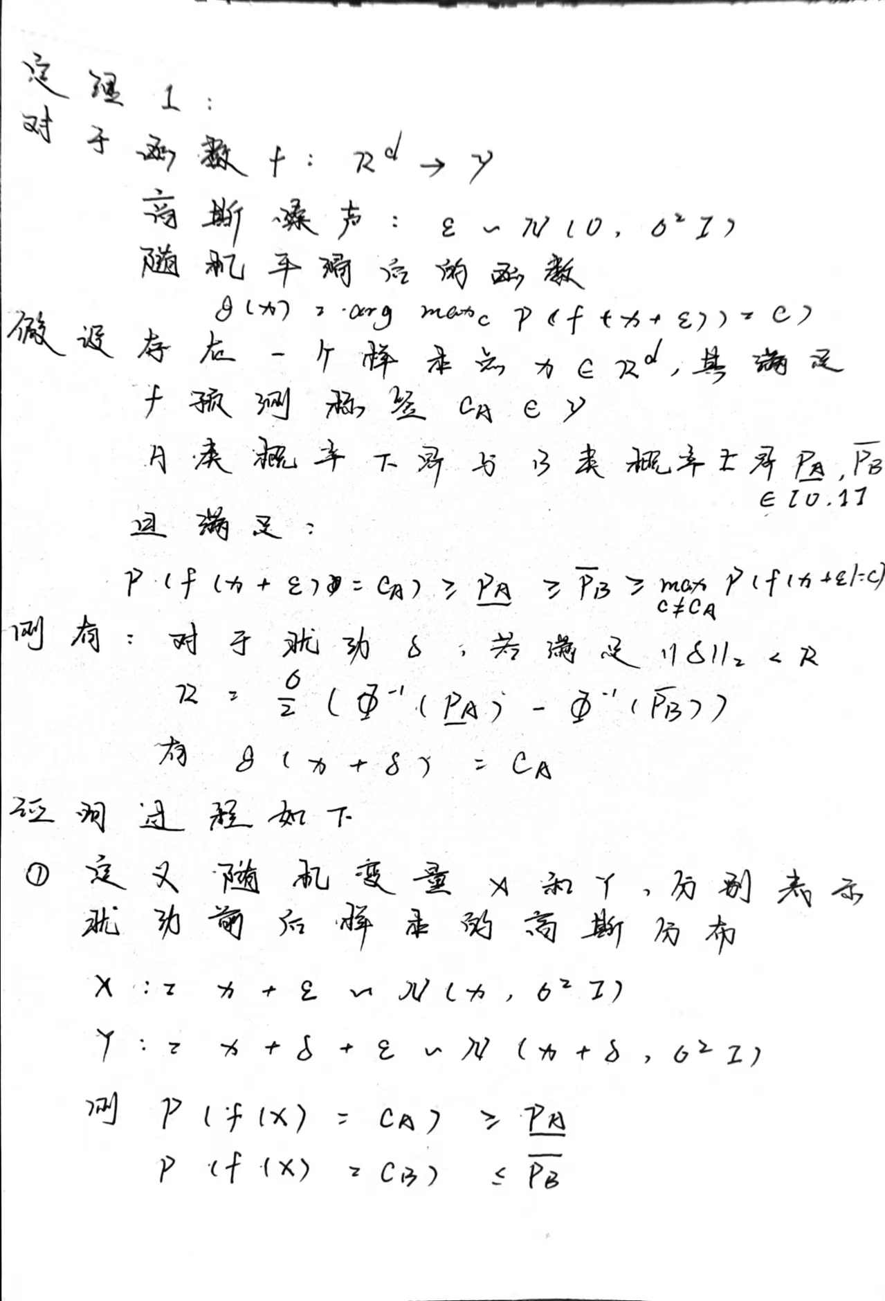
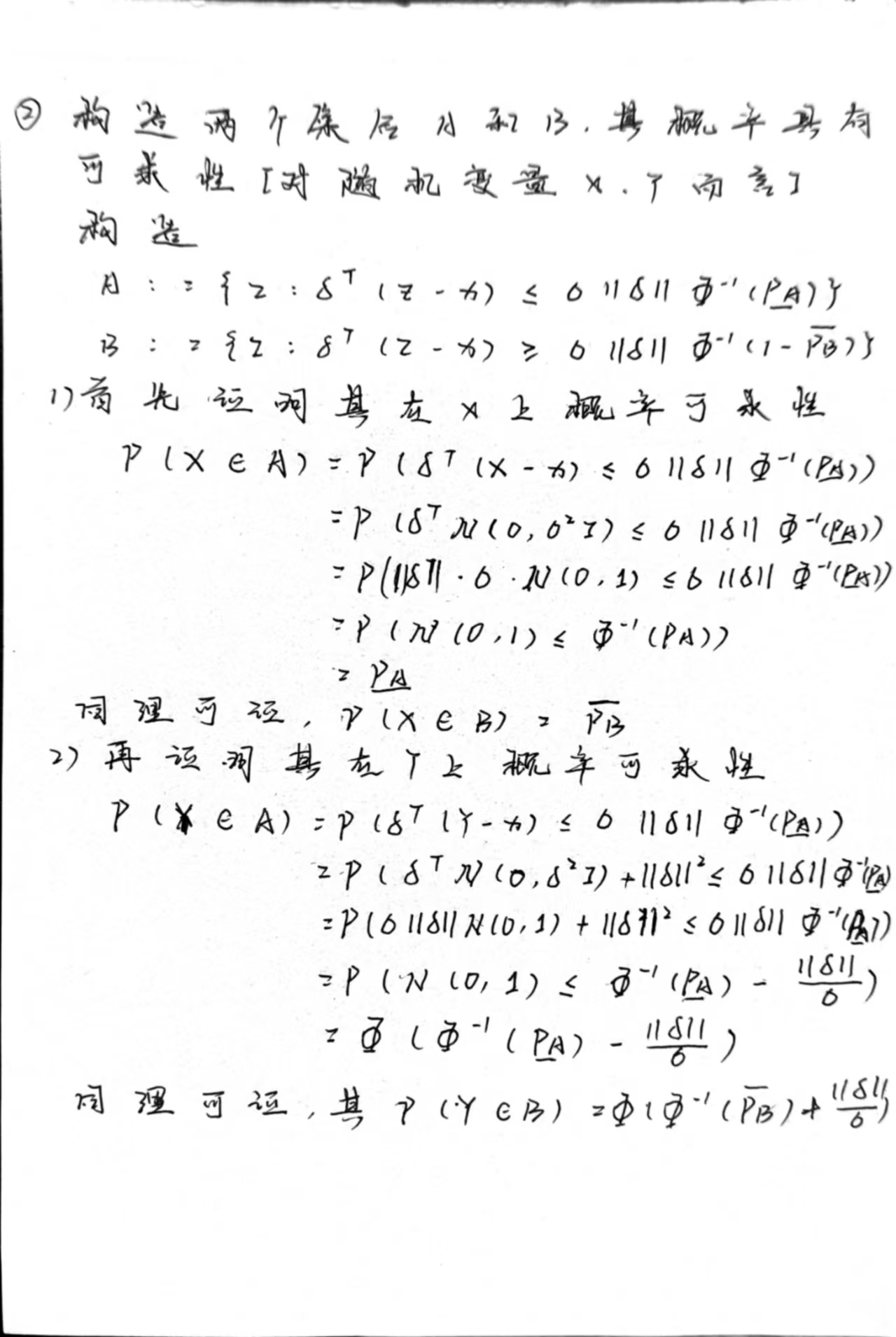
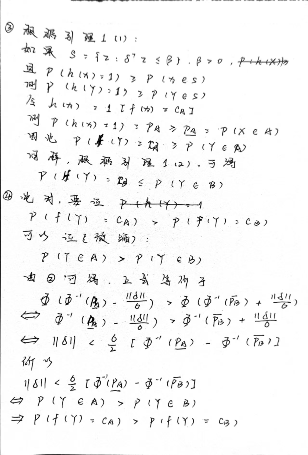
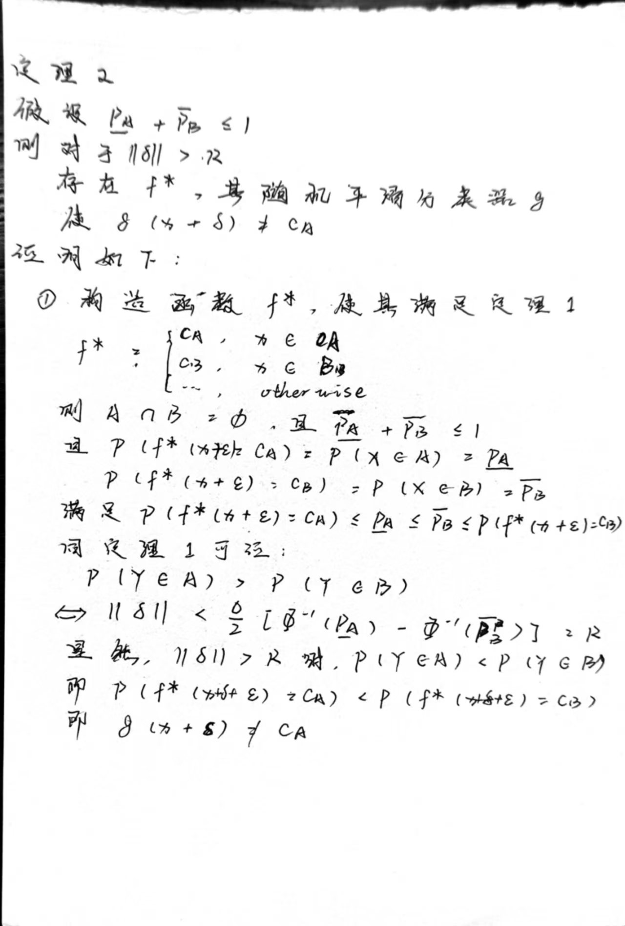
本文与其他以Idea+实验+可解释性为主的论文不同，其以公式推导和数学证明为核心。因此，此笔记不使用往常顺延论文逻辑脉络的写法，意在整理整个推到过程。同时，略去一些引论的证明，只给出最终结论，目的在于突出重点，使论文证明清晰。

第一部分 ： 严密可证对抗鲁棒性

该部分分为两个定理.

定理一证明的是，在扰动小于某个特定半径R的情况下，分类器一定具有鲁棒性。

定理二证明的是，在扰动半径大于该特定半径R的情况下，一定能找到一个特定的f，使平滑后的g不具有鲁棒性。即从函数的角度证明了其严密性。

最终得到的扰动边界为
$$
R = \frac \sigma 2 [\Phi^{-1}(\underline {p_A})-\Phi^{-1}(\overline{p_B})]\
\forall |\delta|<R,g(x+\delta)=c_A\
\forall |\delta|>R,\exist f,g : g(x+\delta)\ne c_A
$$

第二部分 ： 在线性二分类分类器上证明对抗鲁棒性及扩展

第二部分通过四个命题，陈述了可证对抗鲁棒性在线性二分类分类器上的情况。并对无穷半径的情况进行说明。

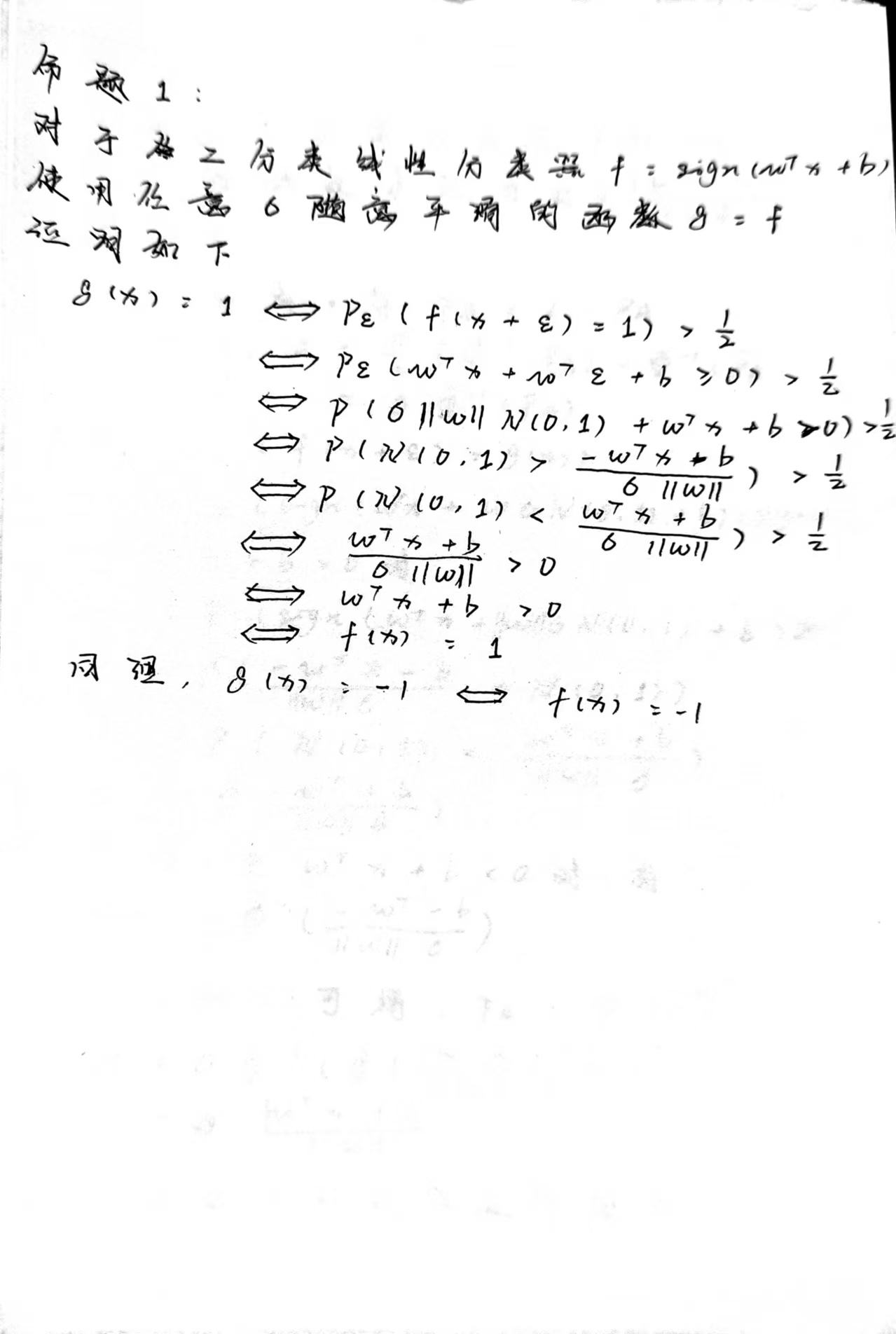
命题一证明 ：对于线性二分类分类器，其随机平滑的结果与原函数一致。

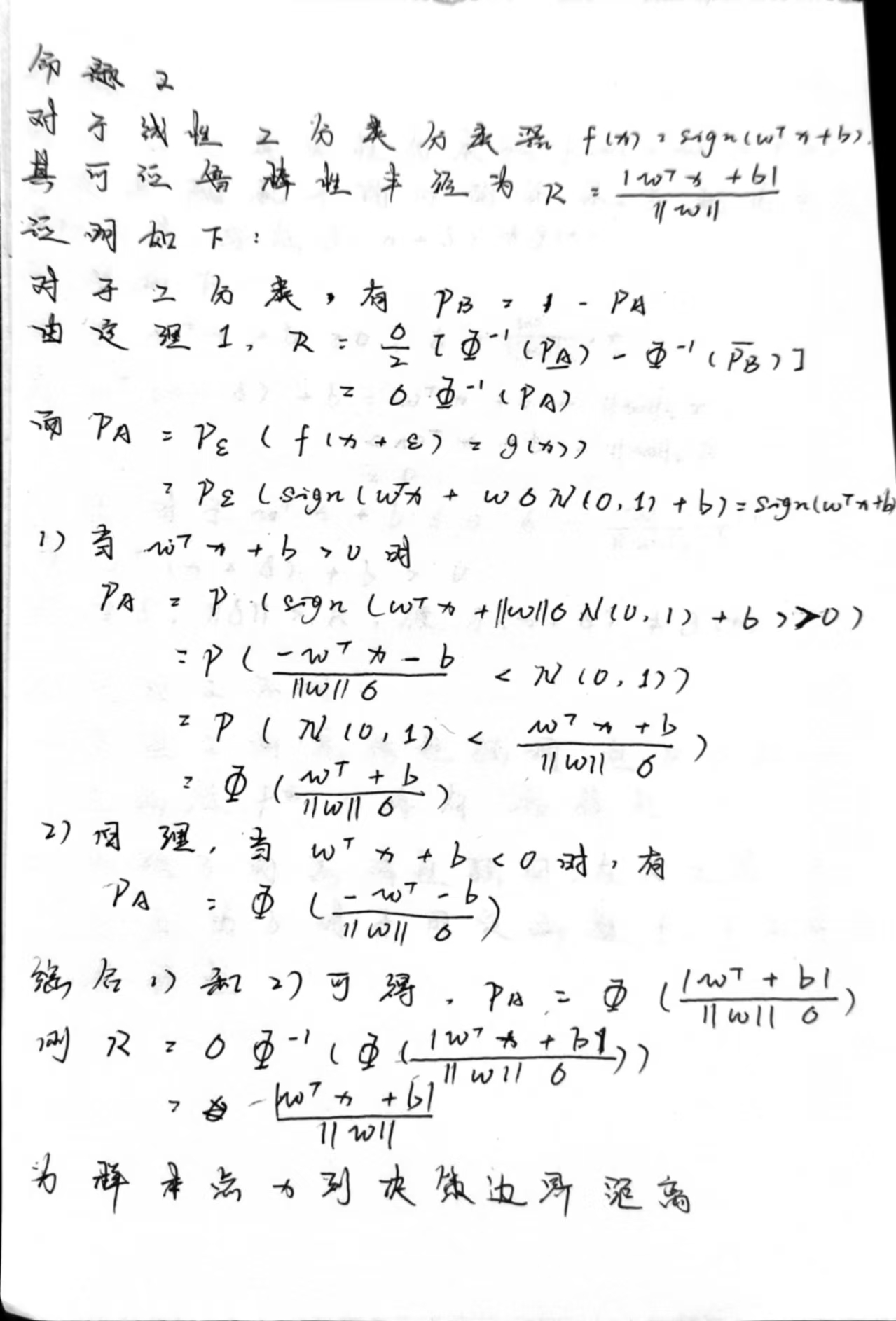
命题二证明 ：对于线性二分类分类器，其扰动半径等于样本点到决策边界的距离，符合实际，佐证了定理一

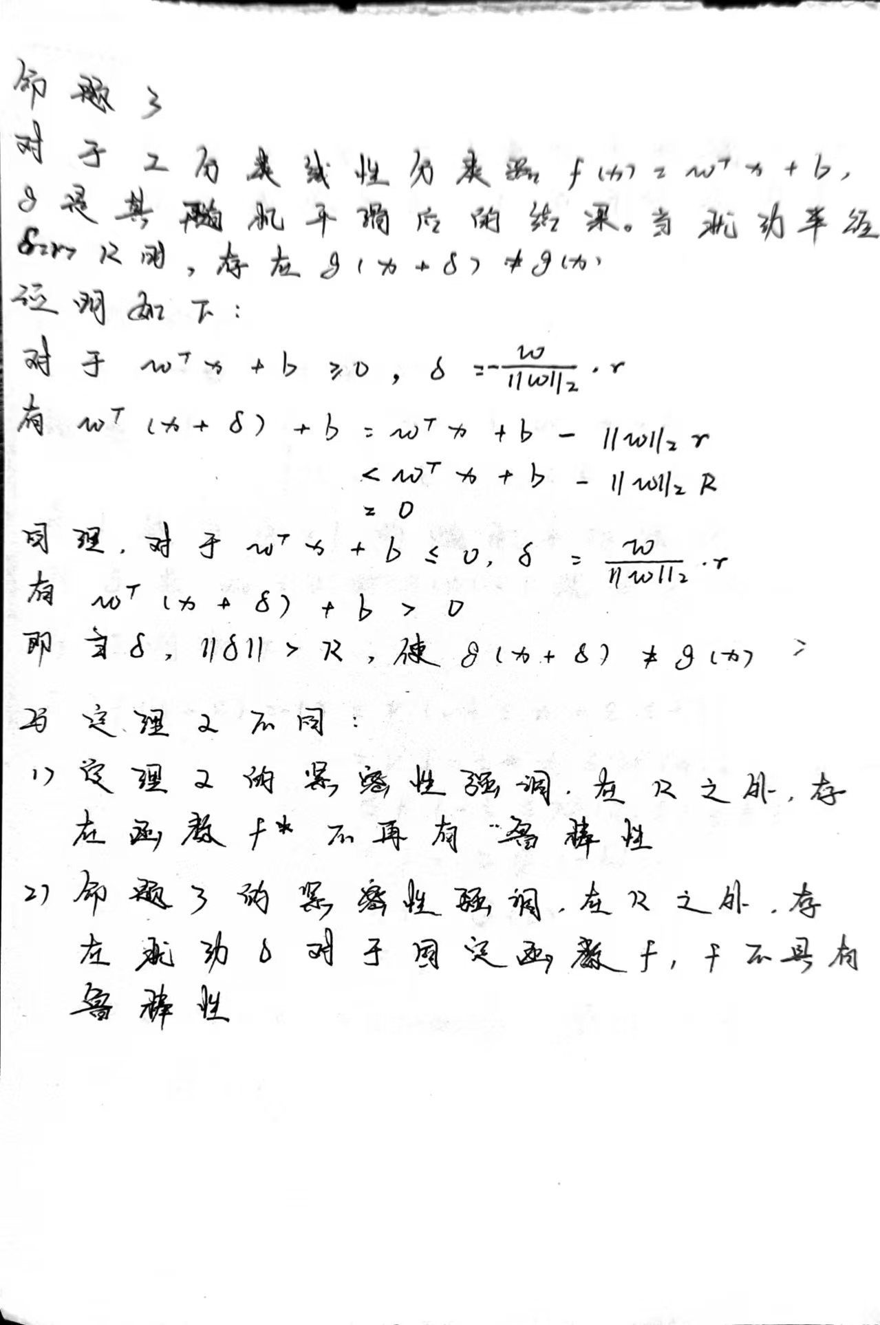
命题三证明 ：线性二分类分类器对于大于扰动半径的扰动，其不再具有鲁棒性。与定理二不同，命题三从“距离”的角度，证明了可证扰动半径的紧密性。

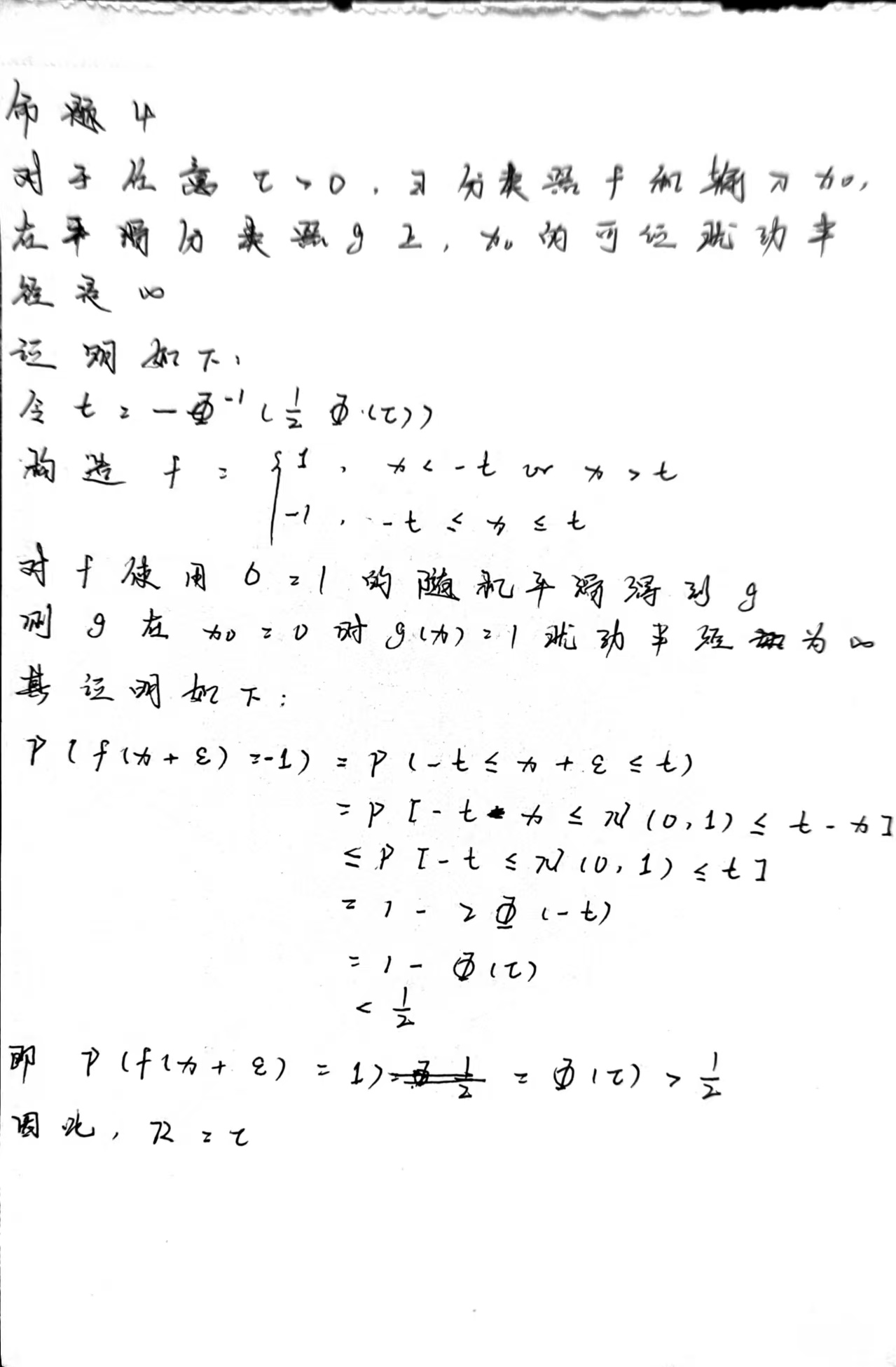
命题四证明 ：存在函数和输入x，使可证扰动半径达到无穷。

命题一

命题二

命题三

命题四

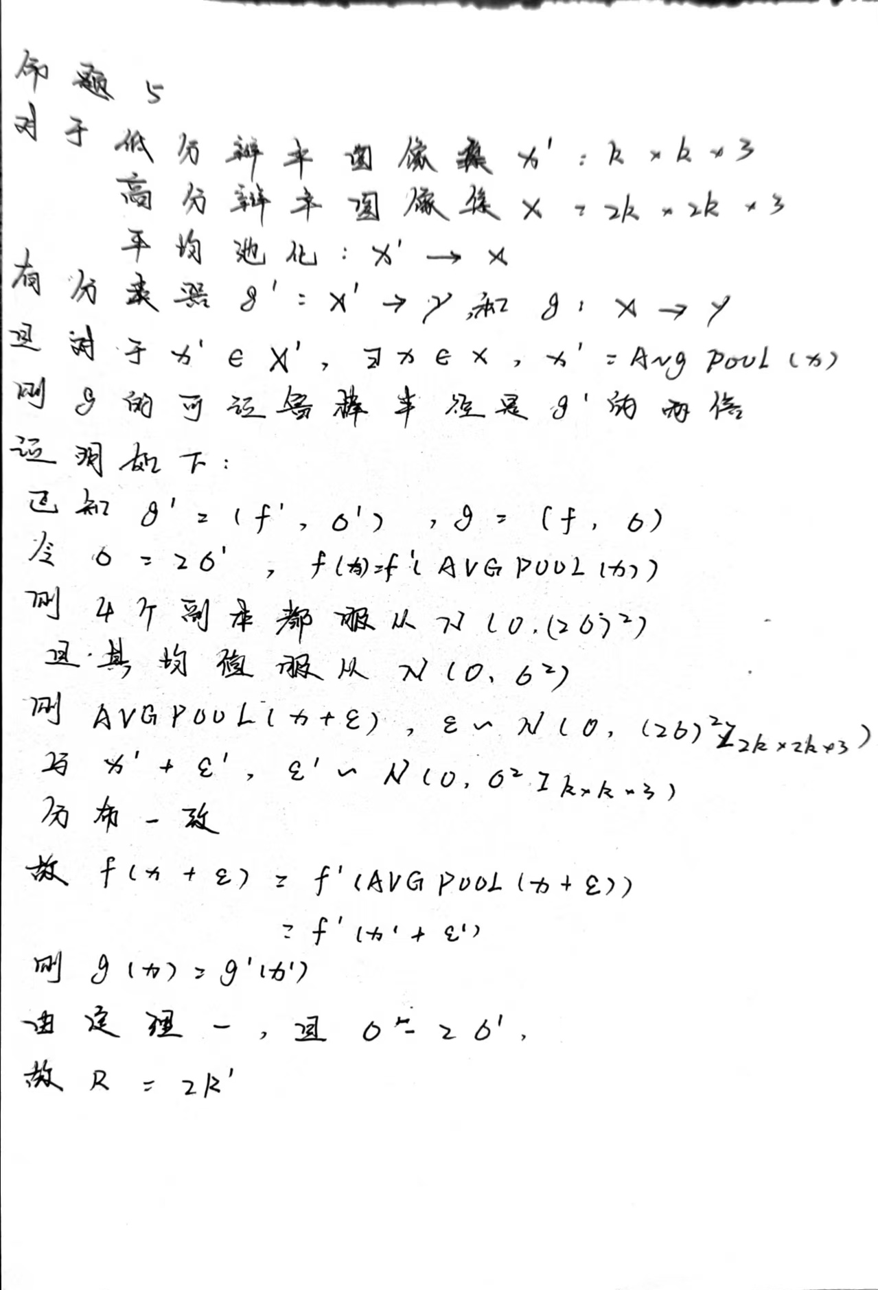
第三部分 ： 可证扰动半径在高分辨率图像的可拓展性

由于可证扰动半径与维度无关，作者额外证明了，在同一张图像高分辨率和低分辨率的情况下，高分辨率具有更高的扰动半径。

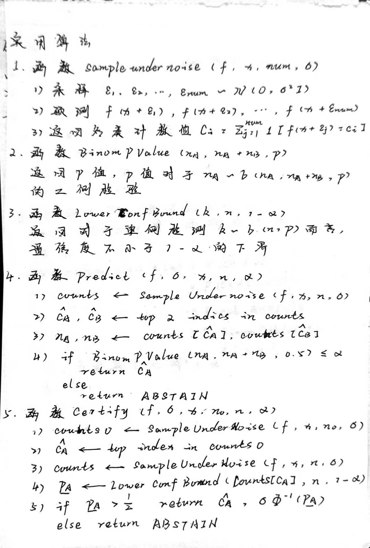
第四部分 ： 针对可证扰动半径提出实用算法

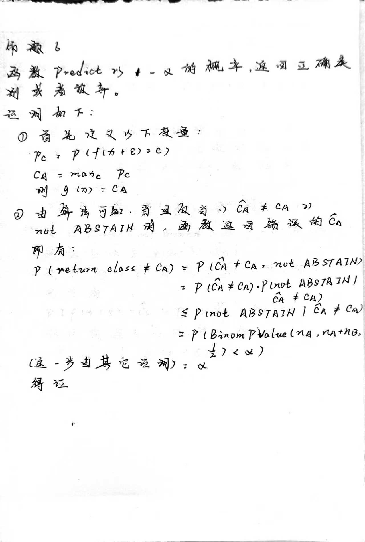
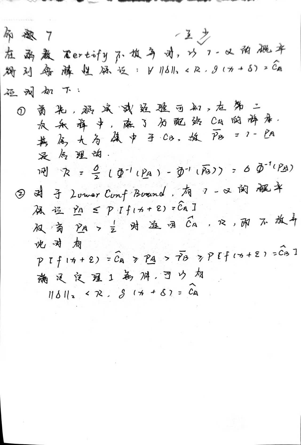
该部分首先提出了实用算法，对于实用算法的“实用性”，命题6和命题7进行了证明。

命题6

命题7

Lec 04 PageRank and Link Analysis

1. PageRank

main idea

Regard links as votes : Page is more important if it has more links

Different Importance of links : links from important links are more important

Combination : A point is important if it is pointed by other important pages

Formula

Common Formulation

$r_i$ : the $i$-th node’s rank or score

$d_i$ : the out-degree of $i$-th node
$$
r_j = \sum_{i->j}\frac{r_i}{d_i}
$$
Matrix Formulation

$A_{ij}$ : equal to 1 if edge from node $i$ to $j$ exists, else 0

$sum_by_row(A)$ : a vector means the out-degrees of nodes in graph

Stochastic adjacency matrix M : if $j->i$, $M_{ij} = 1 / d_j$

$M = (A / sum_by_row(A))^T$

so that $r = M \cdot r$

Eigenvector Formulation

we could regard $r = M \cdot r$ as $1\cdot r = M \cdot r$, so that $r$ would be the eigenvector with the eigenvalue 1

2. How to solve PageRank ?

Power Iteration

algorithm :

1. assign each node an initial page rank

2. repeat until convergence $\sum_i|r_i^{t+1} - r_i^t| <= \varepsilon \Leftrightarrow |r^{t+1}-r^t|_1 <=varepsilon$:
   $$
   \begin{align}
   &r_j^{t+1} = \sum_{i->j} \frac{r_i^t}{d_i}\
   \Leftrightarrow &r = M\cdot r
   \end{align}
   $$

Problem : converge

problem in converge :

dead ends problem : no out-links

Spider traps : all out-links within the group

solution : teleport

At each time step, with the probability $\beta$, follow a link at random; with the probability $1-\beta$, jump to a random node

commonly, $0.8 < \beta <0.9$

Especially, when surfer arrive at a dead end, it has $1.0$ probability to jump to a random node

Formulation as follow (assume that $\sum_{i} r_i = 1$):
$$
\begin{align}
&r_j=\sum_{i\rightarrow j}\beta\frac{r_i}{d_i} + \frac1N(1-\beta)\
\Leftrightarrow &P = \beta \cdot M + \frac1N(1-\beta)
\end{align}
$$

3. Personalized PageRank and Random Walks with Restarts

PageRank, PPR and RWR

difference : the points could be teleported to

PageRank : teleport to anywhere on the graph

PPR : teleport to only a subset of graph

RWR : always teleport to the staring point

Random Walks with Restarts

Idea :

1. Every node has some importance
2. Importance gets evenly split among all edges and pushed to the neighbors

algorithm :

1. Given a set of query_nodes $Q$, randomly select a node $q_i$ and make a random walk
2. make a step to a random neighbor and record visit or with $1 -\beta$ probability to restart from $q_j \in Q$
3. the nodes with the highest visit count have highest proximity to $Q$

1
2
3
4
5
6

item = Q.sample_by_weight()
for i in range(N_STEPS):
	item = item.get_random_neighbor()
    item.visited_time += 1
    if random >= beta :
        item = Q.sample_by_weight()

considers :

• multiple connections
• multiple paths
• directed and undirected connection
• degree of node

4. Matrix Factorization

Embedding and Matrix Factorization

Given : measure the similarity of nodes with adjacency matrix $A$

then : $Z^TZ \approx A$

so that : $\arg \min_Z ||A-Z^TZ||_2$

Exactly : we make matrix factorization of adjacency matrix $A$

Lec 03 Node Embedding

1. Overview

Goal : Efficient task-independent feature learning for ML with graph

Why Embedding ?

1. similarity of embedding space indicate that in origin space
2. encode information
3. could used in many downstream tasks

2. Encoder and Decoder

1
2
3
4
5
6
7
8
9
10
11
12
13
14
15
16
17
18
19
20
21
22
23

graph TB
subgraph Embedding Space
a((ZA))
b((ZB))
c((ZC))
d((ZD))
u((ZU))
v((ZV))
end
subgraph Origin Network
1((A))
2((B))
3((C))
4((D))
5((U))
6((V))
1---2
1---3
1---4
5---1
6---1
end
ARROW[Embedding To]

Learning Node Embedding

1. Encoder maps from nodes to embeddings
2. define a similarity function in origin space
3. Decoder maps from embeddings to similarity scores
4. optimize the parameters of encoder

3. Shallow Encoding : Embedding lookup

$$
Enc(v_i) = z_{v_i} = Z \cdot v_i\
(v_i)_j = \left{ \begin{array}{rcl}
0,i\ne j\
1,i=j
\end{array} \right.\
Z \in R^{d\times |V|}
$$

Weakness : need to optimize a large number of parameters

4. Random Walk : Overview

Algorithm of Random Walk

1. Run short fixed-length random walks starting from each node $u$ with strategy $R$

2. collect $N_R(u)$ for each node $u$, where $N_R(u)$ is a multi-set including all node access in step 1

3. optimize the loss function gradient descent
   $$
   \arg \min_{z_u,u\in V} \sum_{u \in V} \sum_{v \in N_R(u)} - \log \frac{\exp(z_u^Tz_v)}{\sum_{n\in V} z_u^Tz_n}
   $$

Weakness : time expensive

The time complexity of loss function calculating is $O(|N|^2)$, that means it is time expensive

Solution : Negative Sample

To simplify the loss function’s calculating, use the formula as follow
$$
\log \frac{\exp(z_u^Tz_v)}{\sum_{n\in V} z_u^Tz_n} \approx \log (\sigma(z_u^Tz_v)) - \sum_{i=1}^k \log(\sigma(z_u^Tz_{n_i}))\
\sigma(x) = \frac{1}{1+\exp(-x)}\
$$
In the formula, $n_i$ express the node got by sample from random distribution

Proved by the practice, the negative sample have good performance when $k$ just in $[5,20]$

5. The Random Walk Strategy

5.1 Deep Walk

Just run fixed-length, unbiased random walks

Weakness : too constrained

5.2 Node2Vec

Idea : use flexible, biased random walks that can trade off between local and global, where local nodes’ explored by BFS while global by DFS

Super Parameters

1. return parameter $p$ : depend the probability to return to previous node
2. In-out parameter $q$ : depend the probability to BFS or DFS

Example For node2vec

For the graph below, assume previous node is $A$ and current node is $B$

1
2
3
4
5
6
7
8
9
10
11
12
13
14

graph LR
1((A))
subgraph Distance1
2((B))
3((C))
end
subgraph Distance2
5((E))
6((F))
end
1---2
1---3
2---5
2---6

The next node would depend by random sample from the distribution as follow :
$$
nextnode = \left{\begin{array}{rcl}
A,prob = 1 / p\
C,prob = 1 / q\
E,prob = 1\
F,prob = 1
\end{array}\right.\
$$
Attention : the probabilities is not normalized

6. Entire Graph Embedding

6.1 Sum or average

algorithm :

1. run a standard node embedding technique on graph G
2. sum or average all node embeddings in the G

6.2 Virtual Node

algorithm :

1. use a virtual node represent the entire graph, maybe have a series of edges with node in the graph
2. run a standard node embedding technique to get the virtual node’s embedding

6.3 Anonymous Walk Embedding : v1

algorithm :

1. run a random walk on the graph $G$
2. anonymization : for each node in a random walk result, replace its name with the index of the first time it occur
3. for all of anonymous walk produced by 2, count the number of all kinds of anonymous walk
4. Embedding $Z_G[i]$ represent the score or probability of $i$-th anonymous walk

the dimension of embedding $Z_G$:

Because the kind number of anonymous walk depend on the length of walk, so the dimension of embedding depend on it too.

How many random walks m do we need?

We want the distribution to have error of more than $\varepsilon$ with probability less than $\delta$
$$
m = \lceil \frac 2 {\varepsilon^2(\log(2^n-2)-\log(\delta))} \rceil
$$

6.4 Anonymous Walk Embedding : v2

signals :

$\eta$ : the number of samples, the “sample” mean the sum of window number could be extracted from all anonymous walk

$Z$ : the embeddings of walks, $z_i$ express $i$-th specific type of anonymous walk

$\Delta$ : the window size

$z_G$ : the embedding of the entire graph $G$

$w_{i,j}$ : the $j$-th anonymous walk in the series sampled starting from node $i$

algorithm :

learn the embeddings of anonymous walks $Z = {z_i|i=1,2,…,\eta}$ as well as $z_G$

a) for each node i, starting from it and sample anonymous walks randomly, get a series of walks called $[w_{i1},w_{i2},…,w_{iT}]$

b) for a window size $\Delta$, learn to predict walks that co-occur
$$
\arg \min_{Z,z_G,b,U} \sum_{i \in G }\sum_{t=\Delta}^{T-\Delta} -\log P(w_{i,t}|{w_{i,t-\Delta},w_{i,t-\Delta+1},…,w_{i,t+\Delta},z_G})\
P(w_{i,t}|{w_{i,t-\Delta},w_{i,t-\Delta+1},…,w_{i,t+\Delta},z_G}) = \frac{\exp(y(w_{i,t}))}{\sum_{j=1}^\eta \exp(y(w_j))}\
y(w) = b + U (cat(\frac 1 {2\Delta}\sum_{i=-\Delta}^\Delta z_i,z_G))
$$

7. How to use Embeddings

• Clustering by point $z_i$

  • community detection

• Node classification by point $z_i$

  • predict the label of node

• Link prediction : predict edge $(i,j)$ based on $(z_i,z_j)$

  • concatenate : $[z_i,z_j]$
  • Hadamard : $z_i * z_j$
  • Sum / Avg : $z_i + z_j$
  • Distance : $||z_i-z_j||_2$

• Graph classification by $z_G$

Lec 02 Traditional feature-base method for GNN

1. Node-Level Feature

Node Degree

category : importance-based, structure-based

weakness : treat all neighboring nodes equally

Node Centrality

category : importance-based

core : take the node importance in a graph

eigenvector centrality

core : v is important if its neighboring nodes are important

formula :
$$
\begin{align}
&c_v = \frac{1}{\lambda} \sum_{u\in N(v)} c_u\

\Leftrightarrow&\lambda c = A c
\end{align}
$$

bewteeness centrality

core : v is important if v lies on many shortest paths between two nodes

formula :

use $p(u,v)$ express the number of shortest path between $u$ and $v$

use $p(v,s,t)$ express the number of shortest path between $s$ and $t$ via $v$
$$
c_v = \sum_{v\ne s\ne t}\frac{p(s,t)}{p(s,t,v)}
$$

closeness centrality

core : v is important if v has small shortest path lengths to all other nodes

formula :

use $p(u,v)$ express the shortest path length between node $u$ and $v$
$$
c_v = \frac 1 {\sum_{u\ne v}p(u,v)}
$$

Clustering coefficient

category : structure-based

formula :

use $e(N(v))$ express the number of edge among $N(v)$
$$
c_v = \frac{e(N(v))}{C_{k_v}^2}
$$

Graphlet Degree Vector

category : structure-based

core : use the number of graphlet with node $v$ express $v$’s feature

2. Link-Level Feature

Task of Link Prediction

Given : existing links

Aim : predict new links

Key : design features to express a pair of nodes

Formulations of link predictions

links missing at ramdon

core : self-supervised

methodology :

1. remove links randomly
2. predict them

links over time

core : self-regression

Given : $G[t_0,t_0’]$ express graph $G$ at time $t_0’$

Output : $L$ express a list of links that be predicted to appear at time $t_1’$

Evaluation : take top $n$ links in $L$ and then count how many links in it appear at time $t_1’$

Methodology :

1. for each $(x,y)$, compute its score $c(x,y)$
2. decreasing score $c(x,y)$
3. select top $n$ as predicted links

Distance-based Feature

mainly include : shortest path distance between two nodes

use $s(u,v)$ express the length of shortest path between node $u$ and node $v$, and use $s(u,v)$ as the feature of $(u,v)$

weakness : ignore the neighborhood’s degree

Local Neighborhood Overlap

common neighborhood

$|N(v_1)\cap N(v_2)|$

Jaccard’s coefficient

$\frac{|N(v_1)\cap N(v_2)|}{|N(v_1)\cup N(v_2)|}$

Adamic-Adar index

encoding the node importance also

$\sum_{u\in N(v_1)\cap N(v_2)} \frac 1{\log(k_u)}$

Limitation : metric will be 0 if two nodes has no common neighbors but they may connected in the furture

Global Neighborhood Overlap

core : use the number of paths of all lengths between given nodes

calculation : calculate by the power of Adjacency Matrix

Katz index’s formulation :
$$
s_{u,v} = \sum_{l=1}^{\infty} \beta^l A^l\
S = (I-\beta A)^{-1}-I\
where\ 0< \beta < 1
$$

3. Graph-Level Feature

Kernel Methods

Idea : design kernel instead of feature vector

Introduction :

1. $K(G,G’)$ measures the similarity between $G$ and $G’$

2. Kernel metrix $k=(K(G,G’))_{G,G’}$ must be positive semidefinite

3. exists a feature represent $\phi(\cdot)$ such that $K(G,G’) = \phi(G) \phi(G’)$

Core Idea of Graph Kernels

Bags-of-words is the main idea use in graph feature

Graphlet Features

Main Idea : Bags of Graphlets

Given : graph $G$, graphlet list $G_k = (g_1,g_2,…,g_{n_k})$, graphlet count vector $f_G \in R^{n_k}$, where $(f_G)_i = #(g_i \in G)$

Output : $K(G,G’) = f_G^T f_{G^{‘}}$

Problem : if $G$ and $G’$ has different sizes, that woudl greatly skew value

Solutions : normalization by $h_G = \frac{f_G}{sum(f_G)}$ and $K(G,G’) = h_G^T h_{G^{‘}}$

Limitations : NP-hard problem, time expensive

Weisfeiler-Lehman Kernel

Idea ：use neighborhood structure to iteratively enrich node vocabulary, or bags of colors

Methodology :

1. Given graph G with node set V

2. Init : $c^0(v)$

3. for K steps :

   ​ $c^{(k+1)}(v) = hash({c^{(k)}(v),{c^{(k)}(u)}_{u\in N(v)}})$

4. count numbers of nodes with given color

Time Complexity : $K |E|$